AC off-policy

Off-policy Actor Critic

Introduction

• Policy gradient is on-policy, because the gradient ${\nabla }_{\theta }J(\theta )={\mathbb{E}}_{S\sim \mu ,A\sim \pi }[\ast ]$
• We can convert it to off-policy by using importance sampling.

Illustrative Example

Consider a random variable $X\in \mathcal{X}=\{+1,-1\}$. If the probability distribution of $X$ is $p_0$:

$$p_0(X=+1)=0.5p_0(X=-1)=0.5$$

then the expectation of $X$ is

$${\mathbb{E}}_{X\sim p_0}[X]=(+1)\cdot 0.5+(-1)\cdot 0.5=0$$

Question: how to estimate $\mathbb{E}[X]$ by using some samples $\{x_i\}$?

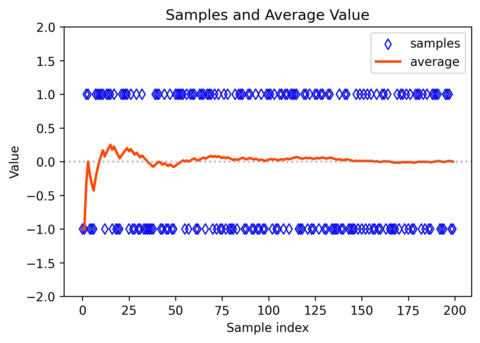
Case 1 (familiar)

The samples $\{x_i\}$ are generated according to $p_0$:

$$\mathbb{E}[x_i]=\mathbb{E}[X]\mathrm{var}[x_i]=\mathrm{var}[X]$$

Then, the average value can converge to the expectation:

$$\bar{x}=\frac{1}{n}\sum _{i=1}^n{x}_i\stackrel{n\to \infty }{\to }\mathbb{E}[X]$$

More

• See the law of large numbers.
• code: Figure Samples Average

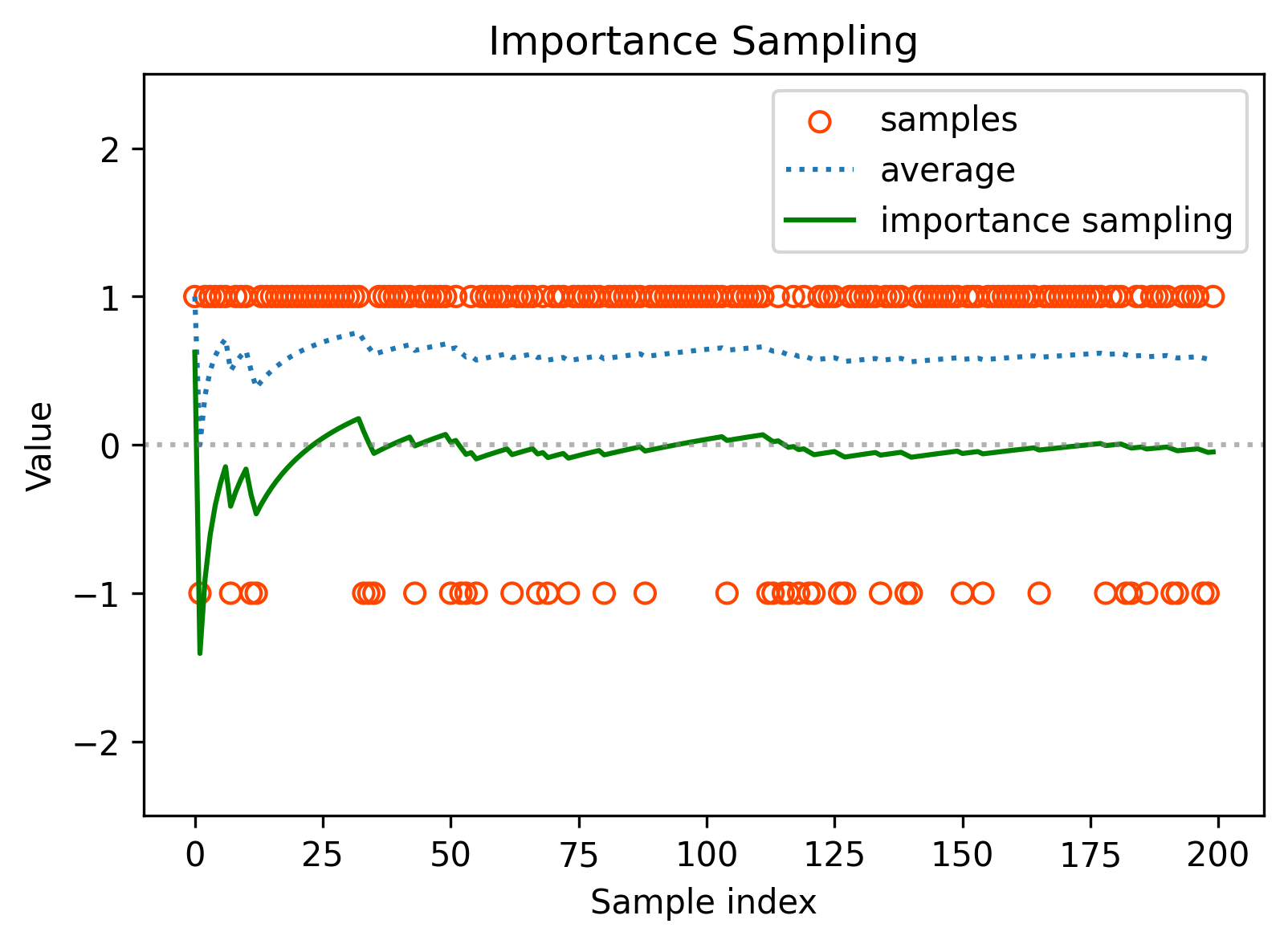
Case 2 (new)

The samples $\{x_i\}$ are generated according to another distribution $p_1$:

$$p_1(X=+1)=0.8p_1(X=-1)=0.2$$

The expectation is

$${\mathbb{E}}_{X\sim p_1}[X]=(+1)\cdot 0.8+(-1)\cdot 0.2=0.6$$

If we use the average of the samples, then without suprising

$$\bar{x}=\frac{1}{n}\sum _{i=1}^n{x}_i\stackrel{n\to \infty }{\to }{\mathbb{E}}_{X\sim p_1}[X]=0.6\ne {\mathbb{E}}_{X\sim p_0}[X]=0$$

Can we use $\{x_i\}\sim p_1$ to estimate ${\mathbb{E}}_{X\sim p_0}[X]$?

• Why to do that? We want to estimate ${\mathbb{E}}_{A\sim \pi }$ where $\pi$ is the target policy based on the sample of a behavior policy $\beta$.(off-policy: get ${\mathbb{E}}_{A\sim \beta }$, want ${\mathbb{E}}_{A\sim \pi }$)
• How to do that? We can’t directly using $\bar{x}$ above, we need to re-weight the samples by the ratio of the target policy and the behavior policy, see Importance sampling.

Importance sampling

Note that

$${\mathbb{E}}_{X\sim p_0}[X]=\sum _x{p}_0(x)x=\sum _x{p}_1(x)\underset{f(x)}{\underbrace{\frac{p_0(x)}{p_1(x)}x}}={\mathbb{E}}_{X\sim p_1}\left[\underset{f(X)}{\underbrace{\frac{p_0(X)}{p_1(X)}X}}\right]$$

Then we can estimate ${\mathbb{E}}_{X\sim p_0}[X]$ by estimating ${\mathbb{E}}_{X\sim p_1}[f(X)]$.

How to estimate ${\mathbb{E}}_{X\sim p_1}[f(X)]$? Easy. Let

$$\bar{f}=\frac{1}{n}\sum _{i=1}^{n}f(x_i),x_i\sim p_1\stackrel{n\to \infty }{\to }{\mathbb{E}}_{X\sim p_1}[f(X)]$$

Therefore, $f$ is a good approximation for ${\mathbb{E}}_{X\sim p_1}[f(X)]={\mathbb{E}}_{X\sim p_0}[X]$.

$${\mathbb{E}}_{X\sim p_0}[X]\approx \bar{f}=\frac{1}{n}\sum _{i=1}^n\underset{f(x_i)}{\underbrace{\frac{p_0(x_i)}{p_1(x_i)}{x}_i}}=\frac{1}{n}\sum _{i=1}^n\underset{\text{importance weight}}{\underbrace{\frac{p_0(x_i)}{p_1(x_i)}}}{x}_i$$

• If $p_1(x_i)=p_0(x_i)$, the importance weight is one and $\bar{f}$ becomes $\bar{x}$.
• If $p_0(x_i)\ge p_1(x_i)$, $x_i$ can be more often sampled by $p_0$ than $p_1$. The importance weight $>1$ can emphasize the importance of this sample, vice versa.

你可能会问：如果都知道 $p_0$和$p_1$了，为什么不直接计算$p_0$的期望呢（还搁这计算$\bar{f}$）？

1. 当x是离散的时候：需要注意的是，我们有时候是获得不了all x的，只能一个一个采样获得x(或者从replay buffer里面采样一个batch)，我们可以用到重要性采样了来更新我们整体的期望。
2. 当x是连续时：比如下一节AC DPG就开始介绍连续action应该怎么做，此时我们要做整个action space空间上的动作概率($\pi ,\beta$)积分是非常困难的，但是如果只是获取某一个特定动作的概率就简单不少（TD，determinisitic），此时我们就可以用重要性采样来对当前的梯度进行修正（$\pi (A|S,\theta )/\beta (A|S)$），更多连续的细节可以参考Sutton书中的13.7节。

TL;DR

一句话总结

当我们用一个分布$p_1$的样本去估计另一个分布$p_0$的期望时，我们需要用$p_0$和$p_1$的比值作为权重来调整样本的平均值。就element-wise的角度而言，我们就是拿将第i个样本除以$p_1(i)$再乘以$p_0(i)$就可以了。

If $\{x_i\}\sim p_1$, then

$$\begin{array}{r}\bar{x}=\frac{1}{n}\sum _{i=1}^n{x}_i\stackrel{n\to \infty }{\to }{\mathbb{E}}_{X\sim p_1}[X]\\ \bar{f}=\frac{1}{n}\sum _{i=1}^n\frac{p_0(x_i)}{p_1(x_i)}{x}_i\stackrel{n\to \infty }{\to }{\mathbb{E}}_{X\sim p_0}[X]\end{array}$$

code: Figure Importance Sampling

Theorem of off-policy policy gradient

• Suppose $\beta$ is the behavior policy that generates experience samples.
• Our goal is to use these samples to update the target policy $\pi$ that can optimize the metric $$J(\theta )=\sum _{s\in \mathcal{S}}{d}_{\beta }(s)v_{\pi }(s)={\mathbb{E}}_{S\sim d_{\beta }}[v_{\pi }(S)]$$ where $d^{\beta }$ is the stationary distribution under policy $\beta$.

In the discounted case where $\gamma \in (0,1)$, the gradient of $J(\theta )$ is

$$\begin{array}{rl}{\nabla }_{\theta }J(\theta )& ={\mathbb{E}}_{S\sim \rho ,A\sim \pi }\left[q_{\pi }(S,A){\nabla }_{\theta }\ln \pi (A|S,\theta )\right]\\ & ={\mathbb{E}}_{S\sim \rho ,A\sim \beta }\left[\frac{\pi (A|S,\theta )}{\beta (A|S)}{q}_{\pi }(S,A){\nabla }_{\theta }\ln \pi (A|S,\theta )\right]\end{array}$$

where $\beta$ is the behavior policy and $\rho$ is the state distribution.

我们这里的$\rho$和之前所提及的on-policy distribution $\mu$做了区分，这里是off-policy的

Algorithm of off-policy actor-critic

The corresponding stochastic gradient-ascent algorithm is

$${\theta }_{t+1}={\theta }_t+{\alpha }_{\theta }\frac{\pi (a_t|s_t,{\theta }_t)}{\beta (a_t|s_t)}(q_t(s_t,a_t)-v_t(s_t)){\nabla }_{\theta }\ln \pi (a_t|s_t,{\theta }_t)$$

Similar to the on-policy case,

$$(q_t(s_t,a_t)-v_t(s_t))\approx r_t+\gamma v_t(s_{t+1})-v_t(s_t)\doteq {\delta }_t(s_t,a_t)$$

Then, the algorithm becomes

$${\theta }_{t+1}={\theta }_t+{\alpha }_{\theta }\frac{\pi (a_t|s_t,{\theta }_t)}{\beta (a_t|s_t)}{\delta }_t(s_t,a_t){\nabla }_{\theta }\ln \pi (a_t|s_t,{\theta }_t)$$

Implementation

Compared with Implementation

$$\boxed{\begin{array}{rl}& \text{Algorithm}\text{Off-Policy Actor-Critic with importance sampling}\\ & \text{Initialization: }\\ & \text{Policy π(a∣s,θ) parameters }{\theta }_0,\text{ value function v(s,w) parameters }{w}_0,\\ & \text{given behavior policy }\beta (a|s).{\alpha }_{\theta },{\alpha }_w>0.\\ & \text{For each episode, do:}\\ & \text{Initialize state }{s}_0.\\ & \text{Select action }{a}_0\sim \beta (a|s_0).\\ & \text{While }{s}_t\text{ is not terminal, do:}\\ & \text{Execute }{a}_t\text{, observe }{r}_{t+1},s_{t+1}.\\ & \text{Select }{a}_{t+1}\sim \beta (a|s_{t+1}).\\ & \text{Advantage (TD Error):}\\ & {\delta }_t=r_{t+1}+\gamma v(s_{t+1},w_t)-v(s_t,w_t)\\ & \text{Importance Sampling:}\\ & {\delta }_t=\frac{\pi (a_t|s_t,{\theta }_t)}{\beta (a_t|s_t)}{\delta }_t\\ & \text{Actor (Policy Update):}\\ & {\theta }_{t+1}\leftarrow {\theta }_t+{\alpha }_{\theta }{\delta }_t{\nabla }_{\theta }\ln \pi (a_t|s_t,{\theta }_t)\\ & \text{Critic (Value Update):}\\ & w_{t+1}\leftarrow w_t+{\alpha }_w{\delta }_t{\nabla }_{w}v(s_t,w_t)\\ & s_t\leftarrow s_{t+1},a_t\leftarrow a_{t+1}\end{array}}$$

Later

discrete action space ⇒ continuous action space

Appendix

Figure Samples Average

import numpy as np
import matplotlib.pyplot as plt
 
# Generate random values +1 or -1, with probability 0.5 for each
np.random.seed(1337)  # Set random seed to ensure reproducibility
num_samples = 200
samples = np.random.choice([1, -1], size=num_samples)
 
# Calculate the average
# cumulative_avg = np.cumsum(samples) / np.arange(1, num_samples + 1)
cumulative_avg = np.zeros(num_samples)
mean = 0  # Initial mean
for k in range(1, num_samples + 1):
    mean = mean - (1 / k) * (mean - samples[k - 1])
    cumulative_avg[k - 1] = mean
 
# Create plot
plt.figure(figsize=(6, 4))
plt.scatter(range(num_samples), samples, marker='d', facecolors='none', edgecolors='blue', label="samples")
plt.plot(range(num_samples), cumulative_avg, color='orangered', label="average", linewidth=2)
 
# Turn off grid
plt.grid(False)
 
# Add a gray dashed line at Value = 0
plt.axhline(y=0, color='gray', linestyle=':', alpha=0.6)
 
# Set legend and labels
plt.xlabel("Sample index")
plt.ylabel("Value")
plt.legend()
plt.ylim(-2, 2)
 
plt.title("Samples and Average Value")
# plt.show()
plt.savefig("Figure_Samples_Average.png", dpi=300, bbox_inches='tight')

Figure Importance Sampling

import numpy as np
import matplotlib.pyplot as plt
 
# Generate random values +1 or -1, with probability 0.5 for each
np.random.seed(42)  # Set random seed to ensure reproducibility
num_samples = 200
samples = np.random.choice([1, -1], size=num_samples, p=[0.8, 0.2])
 
# Calculate the average
avg = np.zeros(num_samples)
mean = 0  # Initial mean
for i, sample in enumerate(samples):
    alpha = 1 / (i + 1)
    mean = mean - alpha * (mean - sample)
    avg[i] = mean
 
# Importance sampling
# Calculate the average using importance sampling
avg_imp = np.zeros(num_samples)
mean_imp = 0  # Initial mean
for i, sample in enumerate(samples):
    alpha = 1 / (i + 1)
    # Update the mean using importance sampling
    ratio = 0.5 / (0.8 if sample == 1 else 0.2)
    mean_imp = mean_imp - alpha * (mean_imp - sample) * ratio
    avg_imp[i] = mean_imp
 
# Create plot
plt.figure(figsize=(6, 4))
plt.scatter(range(num_samples), samples, marker='o', facecolors='none', edgecolors='orangered', label="samples")
plt.plot(range(num_samples), avg, label="average", linestyle=':')
plt.plot(range(num_samples), avg_imp, label="importance sampling", color='green')
 
# Turn off grid
plt.grid(False)
 
# Add a gray dashed line at Value = 0
plt.axhline(y=0, color='gray', linestyle=':', alpha=0.6)
 
# Set legend and labels
plt.xlabel("Sample index")
plt.ylabel("Value")
plt.legend()
plt.ylim(-2.5, 2.5)
 
plt.title("Importance Sampling")
# plt.show()
plt.savefig("Figure_Importance_Sampling.png", dpi=300, bbox_inches='tight')