Visualize Matrix

Introduction

这一节作为附录中的一节是有原因的，其原因就在于当时自己在复现赵老师的VF state value的代码时遇到一个问题：如何可视化一个2D的matrix？这个问题看似很简单，但自己在一开始时还真卡住了，自己最开始的可视化效果是类似这样的：

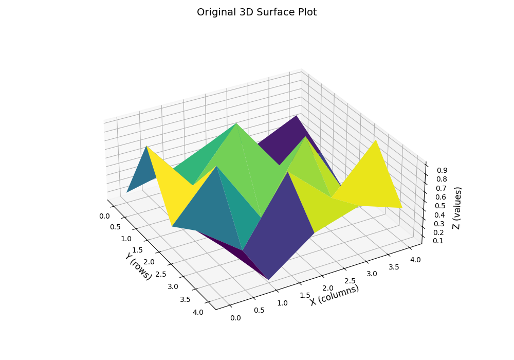
但是这样的效果非常的丑陋，仅仅是由不同的state value的顶点组成的几个平面，并没有很直观的展示出state value的大小关系。所以自己就去问了下deepseek，最终找到了一个比较好的方法，就是使用scipy的RectBivariateSpline来进行线性插值(k=1)，然后再进行可视化。这样的效果就会好很多，如下图所示：

小插曲

DeepSeek一开始给自己的代码是设置了k=3的，给自己生成了曲面的效果，但自己希望的是保留上面原始的平面效果，只是在平面上进行插值，然后自己觉得这种方法是不对的，于是就又分别找了chatgpt和Claude等等模型问了，最后给的答案都没有deepseek好：要么是给自己生成三角化的平面，要么是使用错误的函数，最后自己重新决定看文档，最终发现了RectBivariateSpline这个函数原来是可以线性插值的（k=1）。

当一个东西不work的时候，要非常清楚为什么其不work再找下一个方法，这样起码一直再做减法，不用回溯。

另外得区分一下本章的插值和VF state value的区别，之前的任务的目的是为了估计state value，得到state value附近的值只是一个顺带的效果，而本章的目的是为了可视化一个2D的matrix，就是假设已经得到state value的值了，目的是如何在其周围插值更好。

运用本节的方法，可以可视化之前的结果得到如下的效果：

Smoothed (k=1)	Smoothed (k=2)	Smoothed (k=3)

Results

本章仅仅做展示几个效果，具体的代码可以参考Appendix。

Original	Smoothed (k=1)	Smoothed (k=2)	Smoothed (k=3)

Appendix

复现本节Results中的八张图的代码如下：

python show_matrix.py

# File: show_matrix.py
import numpy as np
import matplotlib.pyplot as plt
from scipy.interpolate import RectBivariateSpline
from pathlib import Path
 
Path("results").mkdir(exist_ok=True)
 
def grid_matrix2d(matrix2d:np.ndarray):
    """
    Generate grid coordinates for 2D matrix visualization
    
    Args:
        matrix2d (np.ndarray): Input 2D numerical matrix
        
    Returns:
        X (np.ndarray): Column coordinate grid matrix with same shape as input matrix
        Y (np.ndarray): Row coordinate grid matrix with same shape as input matrix
        Z (np.ndarray): Original matrix values with unchanged shape
        
    Notes:
        - Uses *ij-indexing* to generate grid, maintains row/column orientation consistent with original matrix
        - X corresponds to column indices, Y corresponds to row indices (opposite of conventional Cartesian system)
        - Returned grid coordinates can be directly used for matplotlib 3D surface plotting
    """
    m, n = matrix2d.shape
    y = np.arange(m)
    x = np.arange(n)
    Y, X = np.meshgrid(y, x, indexing='ij')
    return X, Y, matrix2d
 
def smooth_grid_matrix2d(matrix2d:np.ndarray, k:int, n_points:int):
    """
    Perform bilinear interpolation smoothing on a 2D matrix
    
    Args:
        matrix2d (np.ndarray): Input 2D numerical matrix
        k (int): Interpolation order, default=1 (bilinear interpolation), increase for higher-order interpolation
        n_points (int): Number of interpolation points per dimension
    
    Returns:
        X_new (np.ndarray): Interpolated column coordinate grid matrix (2D array)
        Y_new (np.ndarray): Interpolated row coordinate grid matrix (2D array)
        Z_new (np.ndarray): Interpolated value matrix (2D array)
    
    Notes:
        - Uses SciPy's `RectBivariateSpline` for bivariate spline interpolation
        - Maintains ij-indexing coordinate system where X corresponds to column direction, Y to row direction (opposite of conventional Cartesian system)
        - `grid=True` parameter ensures return of 2D grid format data, directly usable for 3D surface plotting
        - Interpolated grid points are evenly distributed within original matrix coordinate range
        - Example: When n_points=100, generates a 100x100 smooth grid
    """
    m, n = matrix2d.shape  # Get number of rows and columns
 
    # Generate original row and column coordinates (x for columns, y for rows)
    y_orig = np.arange(m)
    x_orig = np.arange(n)
    
    # Create bilinear interpolation function
    interp_func = RectBivariateSpline(y_orig, x_orig, matrix2d, kx=k, ky=k)
 
    # Generate dense interpolation points (using n_points points in this example)
    y_new = np.linspace(0, m-1, n_points)
    x_new = np.linspace(0, n-1, n_points)
 
    # Calculate interpolated Z values
    Z_new = interp_func(y_new, x_new, grid=True)
 
    # Generate grid point coordinates
    Y_new, X_new = np.meshgrid(y_new, x_new, indexing='ij')
 
    return X_new, Y_new, Z_new
 
def draw_matrix2d(matrix2d:np.ndarray, title:str):
    X, Y, Z = grid_matrix2d(matrix2d)
    
    # Draw 3D surface plot
    fig = plt.figure(figsize=(10, 7))
    ax = fig.add_subplot(111, projection='3d')
    surf = ax.plot_surface(Y, X, Z, cmap='viridis', edgecolor='none')
    
    # Set aspect ratio
    ax.view_init(elev=30, azim=330)
    ax.set_box_aspect([2.5, 2.5, 1])
    
    # Set axis labels
    ax.set_ylabel('X (columns)', fontsize=12)
    ax.set_xlabel('Y (rows)', fontsize=12)
    ax.set_zlabel('Z (values)', fontsize=12)
    ax.set_title(title, fontsize=14)
 
    # Add color bar
    # fig.colorbar(surf, ax=ax, shrink=0.5, aspect=5)
    plt.tight_layout()
    plt.savefig(f"results/{title.replace(' ','_')}.png")
 
def draw_matrix2d_smooth(matrix2d:np.ndarray, title:str, k:int, n_points:int=100):
    X, Y, Z = smooth_grid_matrix2d(matrix2d, k, n_points)
 
    # Draw 3D surface plot
    fig = plt.figure(title, figsize=(10, 7))
    ax = fig.add_subplot(111, projection='3d')
    surf = ax.plot_surface(
        Y, X, Z,
        cmap='viridis',
        alpha=0.8,
        edgecolor='none'
    )
 
    # Add gridlines on the interpolated surface
    m, n = matrix2d.shape
    # Draw gridlines along x direction
    for i in range(n):
        # Find the corresponding index in the dense grid
        idx_x = int(i / (n-1) * (n_points-1))
        # Extract the corresponding slice from Z
        ax.plot(Y[:, idx_x], X[:, idx_x], Z[:, idx_x], 
                color='black', linestyle='-', linewidth=1)
    
    # Draw gridlines along y direction
    for j in range(m):
        # Find the corresponding index in the dense grid
        idx_y = int(j / (m-1) * (n_points-1))
        # Extract the corresponding slice from Z
        ax.plot(Y[idx_y, :], X[idx_y, :], Z[idx_y, :], 
                color='black', linestyle='-', linewidth=1)
 
    # Set aspect ratio
    ax.view_init(elev=30, azim=330)
    ax.set_box_aspect([2.5, 2.5, 1])
 
    # Set axis labels
    ax.set_ylabel('X (columns)', fontsize=12)
    ax.set_xlabel('Y (rows)', fontsize=12)
    ax.set_zlabel('Z (values)', fontsize=12)
    ax.set_title(title, fontsize=14)
 
    # Add color bar
    # fig.colorbar(surf, ax=ax, shrink=0.5, aspect=5)
    plt.tight_layout()
    plt.savefig(f"results/{title.replace(' ','_')}.png")
 
def draw_heatmap(matrix2d: np.ndarray, title: str, cmap: str = 'viridis'):
    """Draw a heatmap of a 2D matrix"""
    fig = plt.figure(title, figsize=(8, 6))
    ax = fig.add_subplot(111)
    
    # Use imshow to draw heatmap
    im = ax.imshow(matrix2d, 
                  cmap=cmap,
                  aspect='auto',
                  origin='upper',
                  interpolation='nearest')
    
    # Add color bar
    fig.colorbar(im, ax=ax, shrink=0.8, aspect=10)
    
    # Set axis labels
    ax.set_xlabel('Columns', fontsize=12)
    ax.set_ylabel('Rows', fontsize=12)
    ax.set_title(title, fontsize=14)
    
    # Add grid lines
    ax.grid(visible=True, 
           color='lightgray',
           linestyle='--', 
           linewidth=0.5)
    
    # Set tick positions and labels
    # 设置刻度间隔（每5个点显示一个标签）
    step = max(1, matrix2d.shape[1] // 20)  # 自动计算间隔，至少显示5个标签
    xticks = np.arange(0, matrix2d.shape[1], step)
    ax.set_xticks(xticks)
    ax.set_xticklabels(xticks.astype(int))  # 转换为整数标签
    
    # 对y轴做相同处理
    step_y = max(1, matrix2d.shape[0] // 20)
    yticks = np.arange(0, matrix2d.shape[0], step_y)
    ax.set_yticks(yticks)
    ax.set_yticklabels(yticks.astype(int))
    
    plt.tight_layout()
    plt.savefig(f"results/{title.replace(' ','_')}.png")
 
 
def _test_draw_matrix():
    # Create a 5x5 matrix (example)
    Z = np.random.rand(5, 5)
 
    # Draw the 3D surface plot
    draw_matrix2d(Z, 'Original 3D Surface Plot')
    draw_matrix2d_smooth(Z, 'Smoothed 3D Surface Plot (k=1)', k=1)
    draw_matrix2d_smooth(Z, 'Smoothed 3D Surface Plot (k=2)', k=2)
    draw_matrix2d_smooth(Z, 'Smoothed 3D Surface Plot (k=3)', k=3)
    draw_heatmap(Z, 'Original 2D Heatmap')
    draw_heatmap(smooth_grid_matrix2d(Z,1,100)[2], 'Original 2D Heatmap (k=1)')
    draw_heatmap(smooth_grid_matrix2d(Z,2,100)[2], 'Original 2D Heatmap (k=2)')
    draw_heatmap(smooth_grid_matrix2d(Z,3,100)[2], 'Original 2D Heatmap (k=3)')
    # plt.show()
 
if __name__ == '__main__':
    _test_draw_matrix()