Experiment of Different Basis Functions
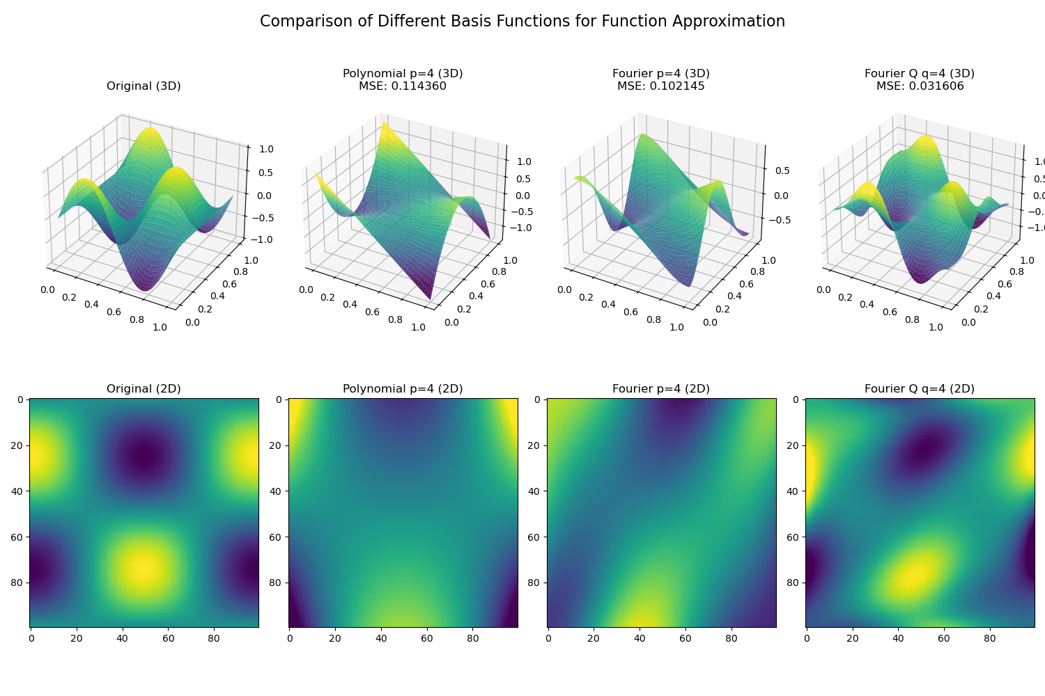
- 我们生成了100x100个网格样本点,每个样本点的坐标为 最终得到的data如上图最左侧的Original (3D)所示
- 我们使用不同的基函数来拟合这个函数,分别是poly_basis和fourier_basis
- poly_basis:最高的degree p=4, 一共有20项,
- fourier_basis:最高的degree p=4, 一共有20项,
- fourierq_basis:这里加了个Q其实只是对项的数目控制不一样,q=4,一共有25项,
- 最终的拟合结果(3D surface和2D heatmap)如上图所示,其中
- 第一列是原始的函数
- 第二列是poly_basis拟合的结果
- 第三列是fourier_basis拟合的结果
- 第四列是fourierq_basis拟合的结果
- 使用numpy的least squeare方法来拟合函数,最终的MSE如下:
- Polynomial basis MSE: 0.114360
- Fourier basis MSE: 0.102145
- Fourier Q basis MSE: 0.031606
- 从拟合的结果来看,fourierq_basis > fourier_basis > poly_basis
Problem
承接之前的VF state value,我们希望有一个特征函数可以比较好的描述状态s,从而可以比较好地将该函数的输出向量线性组合成最终的state value:
这里的主要目的就是研究的表现形式。
该部分主要参考了Sutton书中9.5.1和9.5.2节的内容。
Polynomial basis
Polynomial Basis Definition(From Sutton's book)
Suppose we have state , with each . For a k-dimensional state space, each order-n polynomial-basis feature can be written as
where each is an integer in the set for an integer . These features make up the order-n polynomial basis for dimension k, which contains different features.
For example, we can consider a polynomial basis:
And then we can fit the function using the polynomial basis:
where .
由于后面的阶数会越来越高,如果不限制非常不稳定,所以我们依然会限制
在我们之前的任务中,在grid_world/result.md中的较好结果是使用了,即
结果如下:
| True State Values 3D | TD-Linear(poly-3) Estimated State Values 3D |
|---|---|
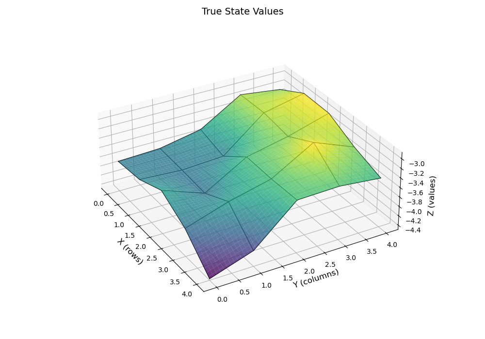 | .png) |
Fourier basis
Fourier Basis Definition(From Sutton's book)
Suppose each state s corresponds to a vector of k numbers, , with each . The th feature in the order- Fourier cosine basis can then be written
where , with for and . This defines a feature for each of the possible integer vectors ci. The inner product has the effect of assigning an integer in to each dimension of . This integer determines the feature’s frequency along that dimension. The features can of course be shifted and scaled to suit the bounded state space of a particular application.
For example, our , then , let , there possible values:
这里记得做一下约束
在我们之前的任务中,在grid_world/result.md中的较好结果也是使用了,即
结果如下:
| True State Values 3D | TD-Linear(fourier-3) Estimated State Values 3D |
|---|---|
| .png) |
Appendix
复现Experiment of Different Basis Functions的结果代码如下(注意这里的代码生成的数据就符合,如果是网格数据的话可以简单将纵横坐标轴的值除以行数和列数,保证为1就可以学到东西了):
python feature.py# File: feature.py
import numpy as np
from matplotlib.colors import Normalize
def pos2poly(state, p=2):
r"""
state: (x,y) or [(x1,y1), (x2,y2), ...]
p: the maximum degree of the polynomial
return: return: poly_basis: [N, (p+1)(p+2)/2]
- [1, x, y, x^2, xy, y^2, ...]
"""
if not isinstance(state, np.ndarray):
state = np.array(state)
if state.ndim == 1:
state = state.reshape(1, -1)
assert state.shape[-1] == 2
n_samples = state.shape[0]
x = state[:, 0]
y = state[:, 1]
features = [np.ones(n_samples)]
for i in range(1, p + 1):
for j in range(i + 1):
# i \in [1, p] j \in [0, i]
# {x^(i-j) * y^j}
features.append((x ** (i - j)) * (y ** j))
return np.column_stack(features)
def pos2fourier(state, p=2):
r"""
state: (x,y) or [(x1,y1), (x2,y2), ...]
p: the maximum degree of the fourier series
return: fourier_basis: [N, (p+1)(p+2)/2]
- [1, cos(\pi x), cos(\pi y), cos(2\pi x), cos(\pi (x+y)), cos(2\pi y), ...]
"""
if not isinstance(state, np.ndarray):
state = np.array(state)
if state.ndim == 1:
state = state.reshape(1, -1)
assert state.shape[-1] == 2
n_samples = state.shape[0]
x = state[:, 0]
y = state[:, 1]
features = [np.ones(n_samples)]
for i in range(1, p + 1):
for j in range(i + 1):
# i \in [1, p] j \in [0, i]
# {cos(\pi (x*(i-j) + y*j))}
features.append(np.cos(np.pi * (x * (i - j) + y * j)))
return np.column_stack(features)
def pos2fourierq(state, q=2):
r"""
state: (x,y) or [(x1,y1), (x2,y2), ...]
q: cos(\pi(c_1 x + c_2 y)), and c_1, c_2 \in {0,...,q}
return: fourier_basis: [N, (q+1)^2]
- [1, cos(\pi x), cos(\pi y), cos(2\pi x), cos(\pi (x+y)), cos(2\pi y), ...]
"""
if not isinstance(state, np.ndarray):
state = np.array(state)
if state.ndim == 1:
state = state.reshape(1, -1)
assert state.shape[-1] == 2
x = state[:, 0]
y = state[:, 1]
features = []
for c1 in range(0, q + 1):
for c2 in range(0, q + 1):
features.append(np.cos(np.pi * (c1 * x + c2 * y)))
return np.column_stack(features)
def _test():
# [1, x, y]
print(pos2poly((1, 2), p=1))
# [1, x, y, x^2, xy, y^2]
print(pos2poly((1, 2), p=2))
print(pos2poly([(1, 2), (3, 4)], p=2))
# [1, cos(\pi x), cos(\pi y)]
print(pos2fourier((1, 2), p=1))
# [1, cos(\pi x), cos(\pi y), cos(2\pi x), cos(\pi (x+y)), cos(2\pi y)]
print(pos2fourier((1, 2), p=2))
print(pos2fourier([(1, 2), (3, 4)], p=2))
# [1, cos(\pi x), cos(\pi y), cos(\pi (x+y))]
print(pos2fourierq((1, 2), q=1))
def _test_fit_curve():
"""
Test function to demonstrate fitting a curve using different basis functions
"""
# Generate some sample data
n_samples = 100
x = np.linspace(0, 1, n_samples)
y = np.linspace(0, 1, n_samples)
grid_x, grid_y = np.meshgrid(x, y)
points = np.column_stack((grid_x.flatten(), grid_y.flatten()))
# Create a target function: z = sin(2πx) * cos(2πy)
z = np.sin(2 * np.pi * grid_x) * np.cos(2 * np.pi * grid_y)
z_flat = z.flatten()
# Fit using polynomial basis
poly_features = pos2poly(points, p=4)
poly_weights = np.linalg.lstsq(poly_features, z_flat, rcond=None)[0]
poly_pred = poly_features @ poly_weights
poly_error = np.mean((poly_pred - z_flat) ** 2)
# Fit using Fourier basis
fourier_features = pos2fourier(points, p=4)
fourier_weights = np.linalg.lstsq(fourier_features, z_flat, rcond=None)[0]
fourier_pred = fourier_features @ fourier_weights
fourier_error = np.mean((fourier_pred - z_flat) ** 2)
# Fit using Fourier Q basis
fourierq_features = pos2fourierq(points, q=4)
fourierq_weights = np.linalg.lstsq(fourierq_features, z_flat, rcond=None)[0]
fourierq_pred = fourierq_features @ fourierq_weights
fourierq_error = np.mean((fourierq_pred - z_flat) ** 2)
print(f"Polynomial basis MSE: {poly_error:.6f}")
print(f"Fourier basis MSE: {fourier_error:.6f}")
print(f"Fourier Q basis MSE: {fourierq_error:.6f}")
# You can add visualization code here if matplotlib is available
try:
import matplotlib.pyplot as plt
title = 'Comparison of Different Basis Functions for Function Approximation'
fig = plt.figure(title, figsize=(15, 10))
fig.suptitle(title, fontsize=16)
# Common colormap and normalization for consistent colors
cmap = 'viridis'
norm = Normalize(vmin=z.min(), vmax=z.max())
kwargs_3d = dict(cmap=cmap, alpha=0.9, norm=norm)
kwargs_2d = dict(cmap=cmap, origin='upper', norm=norm)
# Original function - 3D
ax1 = fig.add_subplot(241, projection='3d')
ax1.plot_surface(grid_x, grid_y, z, **kwargs_3d)
ax1.set_title('Original (3D)')
# Polynomial approximation - 3D
ax2 = fig.add_subplot(242, projection='3d')
ax2.plot_surface(grid_x, grid_y, poly_pred.reshape(n_samples, n_samples), **kwargs_3d)
ax2.set_title(f'Polynomial p=4 (3D)\nMSE: {poly_error:.6f}')
# Fourier approximation - 3D
ax3 = fig.add_subplot(243, projection='3d')
ax3.plot_surface(grid_x, grid_y, fourier_pred.reshape(n_samples, n_samples), **kwargs_3d)
ax3.set_title(f'Fourier p=4 (3D)\nMSE: {fourier_error:.6f}')
# Fourier Q approximation - 3D
ax4 = fig.add_subplot(244, projection='3d')
ax4.plot_surface(grid_x, grid_y, fourierq_pred.reshape(n_samples, n_samples), **kwargs_3d)
ax4.set_title(f'Fourier Q q=4 (3D)\nMSE: {fourierq_error:.6f}')
# Original function - 2D heatmap
ax5 = fig.add_subplot(245)
im5 = ax5.imshow(z.T, **kwargs_2d)
ax5.set_title('Original (2D)')
# Polynomial approximation - 2D heatmap
ax6 = fig.add_subplot(246)
im6 = ax6.imshow(poly_pred.reshape(n_samples, n_samples).T, **kwargs_2d)
ax6.set_title(f'Polynomial p=4 (2D)')
# Fourier approximation - 2D heatmap
ax7 = fig.add_subplot(247)
im7 = ax7.imshow(fourier_pred.reshape(n_samples, n_samples).T, **kwargs_2d)
ax7.set_title(f'Fourier p=4 (2D)')
# Fourier Q approximation - 2D heatmap
ax8 = fig.add_subplot(248)
im8 = ax8.imshow(fourierq_pred.reshape(n_samples, n_samples).T, **kwargs_2d)
ax8.set_title(f'Fourier Q q=4 (2D)')
# Add colorbar
# plt.colorbar(im5, ax=[ax5, ax6, ax7, ax8], shrink=0.8)
plt.tight_layout()
plt.show()
except ImportError:
print("Matplotlib not available for visualization")
if __name__ == "__main__":
_test()
_test_fit_curve()