Stochastic Gradient Descent Convergence Pattern
Pattern and Analysis
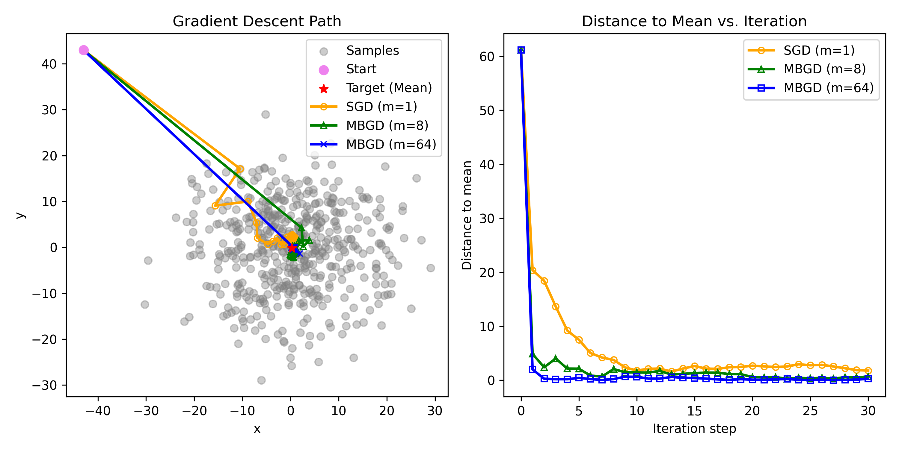
可视化:这里生成了随机500个点,点的分布为N(0,10),这里以较远一个点作为起点(43,43),来通过SGD和Mini-Batch GD(batch_size分别为8和64)来迭代30个iteration,,最后结果如上所示。
观察到
- 即使初始estimate离ture value很远,但是SGD依然可以收敛到ture value的邻居(上图左可以看到一步就收敛到了灰色点聚集区)
- 当estimate越接近真实值时,随机性就表现的越明显,但仍然approaches ture values gradually
下面从相对误差(relative error)的角度来解释这种现象的原因
- 是实际中采样的stochastic gradient
- 是期望的true gradient
- 是相对误差, 表示当前的gradient和期望的gradient的差异
Note that
可以看到我们把相对误差的上界求出来了,而且upper bound 和 成反比,这就解释了:
- 当离越远时,越大,越小,即gradient的估计越准确,SGD behaves like GD
- 当接近时,越小,越大,即gradient的估计越不准确,SGD behaves like random search(exhibits more randomness in the neighborhood of the optimal solution )
Appendix
开头figure的代码如下:
import numpy as np
import matplotlib.pyplot as plt

# Set random seed for reproducible results
np.random.seed(43)

# Generate sample data
n_samples = 500
X = np.random.randn(n_samples, 2) * 10

# Target point (mean)
mean = np.mean(X, axis=0)

# Define gradient descent algorithm
def gradient_descent(X, m, init_w, n_iter=30):
    # Initial value
    w = init_w
    path = [w]

    # span = 10
    # lr = 2 / (span + 1)

    # Simulate gradient descent process
    for i in range(n_iter):
        # Sample from X
        idx = np.random.choice(n_samples, m)
        X_batch = X[idx]
        # w = w - (w - np.mean(X_batch, axis=0)) * lr
        w = w - (w - np.mean(X_batch, axis=0)) / (i + 1)
        path.append(w)
    return np.array(path)

# Run gradient descent multiple times with different m values
# init_w = np.random.randn(2) * 50
init_w = np.array([-43, 43])
path_sgd = gradient_descent(X, m=1, init_w=init_w)
path_mbgd_8 = gradient_descent(X, m=4, init_w=init_w)
path_mbgd_64 = gradient_descent(X, m=32, init_w=init_w)

# Plotting
fig, (ax1, ax2) = plt.subplots(1, 2, figsize=(10, 5))

path_kwargs = dict(
    # alpha=0.8,
    markersize=5,
    linewidth=2,
    markerfacecolor='none'
)

node_kwargs = dict(
    s=50,
    zorder=10,
    # facecolor='none'
)

ax1.scatter(X[:, 0], X[:, 1], label="Samples", color='gray', alpha=0.4)
ax1.scatter(init_w[0], init_w[1], color='violet', label="Start", marker='o', **node_kwargs)
ax1.scatter(mean[0], mean[1], color='red', label="Target (Mean)", marker='*', **node_kwargs)

ax1.plot(path_sgd[:, 0], path_sgd[:, 1], label="SGD (m=1)", color='orange', marker='o', **path_kwargs)
ax1.plot(path_mbgd_8[:, 0], path_mbgd_8[:, 1], label="MBGD (m=8)", color='green', marker='^', **path_kwargs)
ax1.plot(path_mbgd_64[:, 0], path_mbgd_64[:, 1], label="MBGD (m=64)", color='blue', marker='x', **path_kwargs)
ax1.set_title("Gradient Descent Path")
ax1.set_xlabel("x")
ax1.set_ylabel("y")
ax1.legend()

# Second plot: Iteration Steps vs. Distance to Mean
distance_sgd = np.linalg.norm(path_sgd - mean, axis=1)
distance_mbgd_8 = np.linalg.norm(path_mbgd_8 - mean, axis=1)
distance_mbgd_64 = np.linalg.norm(path_mbgd_64 - mean, axis=1)

ax2.plot(range(len(distance_sgd)), distance_sgd, label="SGD (m=1)", color='orange', marker='o', **path_kwargs)
ax2.plot(range(len(distance_mbgd_8)), distance_mbgd_8, label="MBGD (m=8)", color='green', marker='^', **path_kwargs)
ax2.plot(range(len(distance_mbgd_64)), distance_mbgd_64, label="MBGD (m=64)", color='blue', marker='s', **path_kwargs)
ax2.set_title("Distance to Mean vs. Iteration")
ax2.set_xlabel("Iteration step")
ax2.set_ylabel("Distance to mean")
ax2.legend()

plt.tight_layout()
plt.savefig('sgd.png', dpi=300)