Encoder-Free Multimodal Scaling
An interactive field guide
If pixels enter the language decoder directly, where does the visual work go—and when might the extra training cost disappear?
Before this article: ViT · CLIP and SigLIP series · Visual tokenizers in multimodal models
What was already possible
Section titled “What was already possible”What does removing an encoder actually remove?
Section titled “What does removing an encoder actually remove?”Reading: Lin Chen et al., “How Far Are We from Removing the Visual Encoder? Scaling Laws for Encoder-Free Multimodal Pretraining”, arXiv:2609.35457v1, 28 September 2026. The explanation covers the main text and Appendices A–G.
A visual encoder turns image patches into contextual representations before the language decoder sees them. Its pretrained weights supply a visual prior. Encoder-free models keep an input projection, but move representation learning into the decoder. They do not remove visual computation.
This paper asks how that change affects compute allocation. Does an extra unit of budget belong in a larger decoder or in more training tokens? The evidence comes from controlled pretraining sweeps, not from comparing unrelated flagship systems.
Read the result in two parts. Within the measured range, the encoder-free multimodal frontier is worse. Its fitted improvement is faster, which supports a conditional prediction of eventual parity. The second statement is not an observed crossover.
- Paper: §1 — 2609.35457v1
A matched decoder ladder, a fixed-size visual encoder
Section titled “A matched decoder ladder, a fixed-size visual encoder”Both families use 11 sparse MoE decoder sizes: 1.1B–44B total and 71M–2.4B active non-embedding parameters. The first layer is dense. Subsequent layers have 256 routed experts, top-8 activation and one shared expert. Both use RMSNorm and RoPE. Total parameters and active parameters describe different costs.
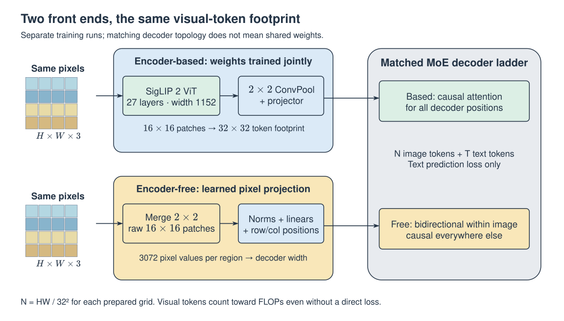
The pixels, preprocessing, data mixture and decoder visual-token count match. One visual token covers a 32×32 pixel region. The pretrained SigLIP 2 encoder is roughly 400M parameters: 27 layers, width 1152, patch size 16 and AnyRes. Its weights are trained jointly with the decoder; only its architecture stays fixed across the ladder.
The study therefore isolates decoder scaling with a fixed-size visual prior. It does not optimize encoder size and decoder size together. The main mask also differs between families; a causal encoder-free ablation checks whether the allocation shift survives this change.
- Paper: Appendix A.1–A.2 — 2609.35457v1
What changes, and why
Section titled “What changes, and why”Select a module inside a blue outline to inspect shapes, equations and pseudocode. You can also use Tab and Enter.
1. Pretrained visual front end
Shape / interface: N16 × 1152 → N × d
For a preprocessed image grid of height H and width W divisible by 32, the ViT first produces HW/256 patch features at width 1152. A 2×2 ConvPool adapter reduces the spatial token count by four. A projector maps the result to decoder width d. Every decoder token then uses causal attention. The ViT has already mixed information bidirectionally inside the image.
features = siglip2(image)             # N16 × 1152
visual = projector(conv_pool_2x2(features))  # N × d
logits = decoder(interleave(text, visual), causal_mask)
loss = cross_entropy(logits[text_targets], targets)
Training state: Joint pretraining; source-based teaching pseudocode, not inspected official code.
Step-by-step explanation: From pretrained visual features to decoder tokens
2. Raw-pixel front end
Shape / interface: N × 3072 → N × h → N × d
The encoder-free branch groups four neighboring 16×16 raw patches into one 32×32 region. Each region contains 3072 scalar pixel values. LayerNorm → linear → LayerNorm transforms that vector; learned row and column embeddings add spatial position. LayerNorm → RMSNorm → linear then maps to the decoder width. The paper does not specify every intermediate width, so h below remains symbolic.
pixels = merge_2x2(raw_patches_16(image))
u = ln2(linear1(ln1(pixels)))
u = u + row_position + column_position
visual = linear2(rmsnorm(ln3(u)))
logits = decoder(interleave(text, visual), image_bidirectional_mask)
Training state: Joint pretraining; source-based teaching pseudocode, not inspected official code.
Step-by-step explanation: Raw pixels still need a trainable front end
3. Decoder attention
Shape / interface: (N + T) × d → text logits
A query can read an earlier key. In the encoder-free main setting it can also read a later key when both positions belong to the same image. This does not expose future text. During text generation, all given image tokens are context; this mask is not a rule for generating pixels. The lab uses two text tokens, four image tokens and two later text tokens.
allow = causal | same_image
loss = CE(logits[text_targets], targets)
Training state: Joint pretraining; source-based teaching pseudocode, not inspected official code.
Step-by-step explanation: Bidirectional inside an image; causal elsewhere
From pretrained visual features to decoder tokens
Section titled “From pretrained visual features to decoder tokens”For a preprocessed image grid of height H and width W divisible by 32, the ViT first produces HW/256 patch features at width 1152. A 2×2 ConvPool adapter reduces the spatial token count by four. A projector maps the result to decoder width d. Every decoder token then uses causal attention. The ViT has already mixed information bidirectionally inside the image.
features = siglip2(image)             # N16 × 1152
visual = projector(conv_pool_2x2(features))  # N × d
logits = decoder(interleave(text, visual), causal_mask)
loss = cross_entropy(logits[text_targets], targets)- Paper: Appendix A.1 — 2609.35457v1
Raw pixels still need a trainable front end
Section titled “Raw pixels still need a trainable front end”The encoder-free branch groups four neighboring 16×16 raw patches into one 32×32 region. Each region contains 3072 scalar pixel values. LayerNorm → linear → LayerNorm transforms that vector; learned row and column embeddings add spatial position. LayerNorm → RMSNorm → linear then maps to the decoder width. The paper does not specify every intermediate width, so h below remains symbolic.
This adapts the Gemma 4 12B Unified input recipe, but changes its 3×3 patch merging to 2×2 for the comparison. Copying the original 48×48 token footprint would break the matched token count. For multiple AnyRes grids, apply this shape reasoning to each prepared grid.
pixels = merge_2x2(raw_patches_16(image))
u = ln2(linear1(ln1(pixels)))
u = u + row_position + column_position
visual = linear2(rmsnorm(ln3(u)))
logits = decoder(interleave(text, visual), image_bidirectional_mask)- Paper: Appendix A.1 — 2609.35457v1
Read Figure 2
Section titled “Read Figure 2”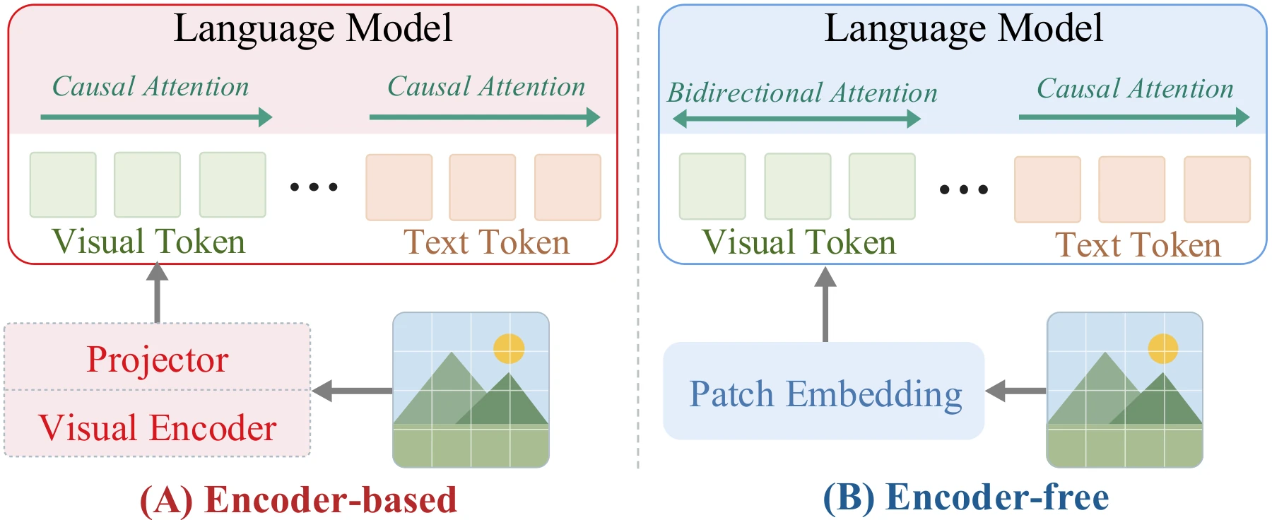
Bidirectional inside an image; causal elsewhere
Section titled “Bidirectional inside an image; causal elsewhere”A query can read an earlier key. In the encoder-free main setting it can also read a later key when both positions belong to the same image. This does not expose future text. During text generation, all given image tokens are context; this mask is not a rule for generating pixels. The lab uses two text tokens, four image tokens and two later text tokens.
- Paper: §2.3, §3.3 — 2609.35457v1
Work through the mechanism
Section titled “Work through the mechanism”Count what is processed, not just what is supervised
Section titled “Count what is processed, not just what is supervised”C is objective-specific training FLOPs, M is decoder FLOPs per processed token and D is the processed token count. Visual positions are excluded from cross-entropy but included in multimodal D. Attention cost also depends on packed length and the mask, so equal token counts do not imply identical M. M is not the total MoE parameter count.
The main plots count decoder compute. Appendix C adds the current visual front-end training cost and preserves the qualitative allocation ordering. That addition does not price the historical SigLIP 2 pretraining. Neither convention establishes full lifecycle cost or measured hardware latency.
- o
- Text or multimodal objective
- s
- Encoder-free or encoder-based family
- ℓ
- Mean packed sequence length for the objective
- Paper: §2.4; Appendix C — 2609.35457v1
An IsoFLOP curve asks where one budget goes
Section titled “An IsoFLOP curve asks where one budget goes”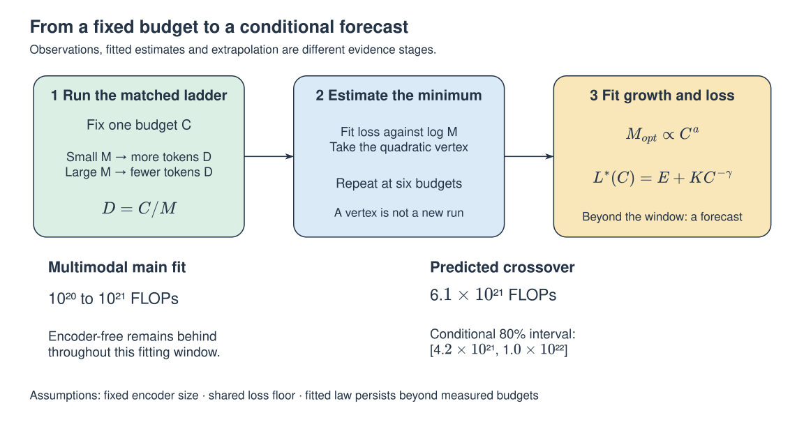
Hold C fixed, choose decoder scales M, and allocate D=C/M tokens to each. Too small a model leaves a capacity bottleneck; too large a model gets too few tokens. Fit validation loss as a quadratic in log M and use its minimum. Repeating this process across budgets gives allocation laws and a loss frontier. A fitted minimum is an estimate, not another training run.
Each objective uses six logarithmically spaced budgets. The text window is 2×10¹⁹–2×10²⁰ FLOPs; the multimodal window is 10²⁰–10²¹. Exponents describe growth within each model family. The normalized lab uses each family’s own value at the smallest budget as 1, so its lines cannot compare absolute model sizes.
| Objective / family | a | b | γ |
|---|---|---|---|
| Text / Free | 0.427 | 0.573 | 0.0973 |
| Text / Based | 0.422 | 0.578 | 0.0979 |
| Multimodal / Free | 0.570 | 0.430 | 0.3778 |
| Multimodal / Based | 0.464 | 0.536 | 0.2998 |
- Paper: Appendix A.5 — 2609.35457v1
- Paper: Table 2: IsoFLOP estimates — 2609.35457v1
Derive the optimum before interpreting the exponents
Section titled “Derive the optimum before interpreting the exponents”For the separable approximation L=E+AM⁻ᵅ+BD⁻ᵝ, substitute D=C/M. Differentiate with respect to M. The stationary point balances the two marginal loss terms, not necessarily their raw magnitudes. Solving gives a=β/(α+β), b=α/(α+β) and γ=αβ/(α+β). The paper estimates allocation exponents from the IsoFLOP profiles; this derivation explains the model behind its overtraining analysis.
A larger multimodal a means more of a growing budget goes into decoder scale. It does not say “57% of all FLOPs buy parameters”. At ten times the budget, a=0.570 means about 3.72× the baseline M and 2.69× its D.
- Paper: Appendix D — 2609.35457v1
Equal loss, two different efficiency ratios
Section titled “Equal loss, two different efficiency ratios”Use encoder-free as target and encoder-based as reference. EGᶜ compares the compute needed to reach the same loss; EGᴹ compares the selected FLOPs per token at that loss. A value below 1 is unfavorable to encoder-free. For example, EGᴹ=0.80 implies 1/0.80=1.25 times as many FLOPs per token, not 20% fewer parameters.
- Paper: §2.2; §3.2 — 2609.35457v1
Explore the allocation law
Each family starts at its own baseline. Curves show an analytical law, not training observations. Solid lines cover the paper’s fitting window; dashed lines extend that law. The dots mark your selected budget, not measured runs.
1.00× budget · 1.00e+20 decoder FLOPs · within fitting window
● Encoder-free● Encoder-based
| Family | a | M / M₀ | D / D₀ |
|---|---|---|---|
| Encoder-free | 0.570 | 1.0000 | 1.0000 |
| Encoder-based | 0.464 | 1.0000 | 1.0000 |
At the 10× boundary, the multimodal free branch grows to 3.7154× M and 2.6915× D. Their product is 10. Separate normalization does not imply equal starting capacities or equal losses. Source: Table 2, decoder-only accounting.
Inspect the attention mask
T denotes text; I denotes four positions in one image. Rows are queries, columns are keys. A dot means the key is visible. This is a structural example, not measured attention weights.
| Q / K | T0 | T1 | I0 | I1 | I2 | I3 | T2 | T3 |
|---|---|---|---|---|---|---|---|---|
| T0 | ● | – | – | – | – | – | – | – |
| T1 | ● | ● | – | – | – | – | – | – |
| I0 | ● | ● | ● | ● | ● | ● | – | – |
| I1 | ● | ● | ● | ● | ● | ● | – | – |
| I2 | ● | ● | ● | ● | ● | ● | – | – |
| I3 | ● | ● | ● | ● | ● | ● | – | – |
| T2 | ● | ● | ● | ● | ● | ● | ● | – |
| T3 | ● | ● | ● | ● | ● | ● | ● | ● |
I0 can read: T0, T1, I0, I1, I2, I3.
The first image query gains three later image keys. It still cannot read T2 or T3. Text queries remain causal in both modes. Later text can read all preceding image positions. The experiment does not run a model or generate pixels.
Training and experimental evidence
Section titled “Training and experimental evidence”The crossover is beyond the main fitting window
Section titled “The crossover is beyond the main fitting window”The main multimodal fit ends at 10²¹ FLOPs. Its predicted parity point is 6.1×10²¹ FLOPs. The table gives conditional central 80% bootstrap intervals, not a guarantee that a new run will cross inside them. The law must persist, the encoder size stays fixed, and both families share an irreducible loss floor.
Topic-level fits predict earlier parity on STEM and then Charts, with later parity on GUI, OCR and Caption. That is a forecast over validation topics. It is not evidence that all chart benchmarks already favor encoder-free.
| Regime | Predicted FLOPs | Conditional 80% interval |
|---|---|---|
| k=1 | 6.1×10²¹ | [4.2×10²¹, 1.0×10²²] |
| k=5 | 1.2×10²² | [8.4×10²¹, 2.0×10²²] |
- Paper: §3.2 — 2609.35457v1
- Paper: Appendix B.4 — 2609.35457v1
Read Figure 4
Section titled “Read Figure 4”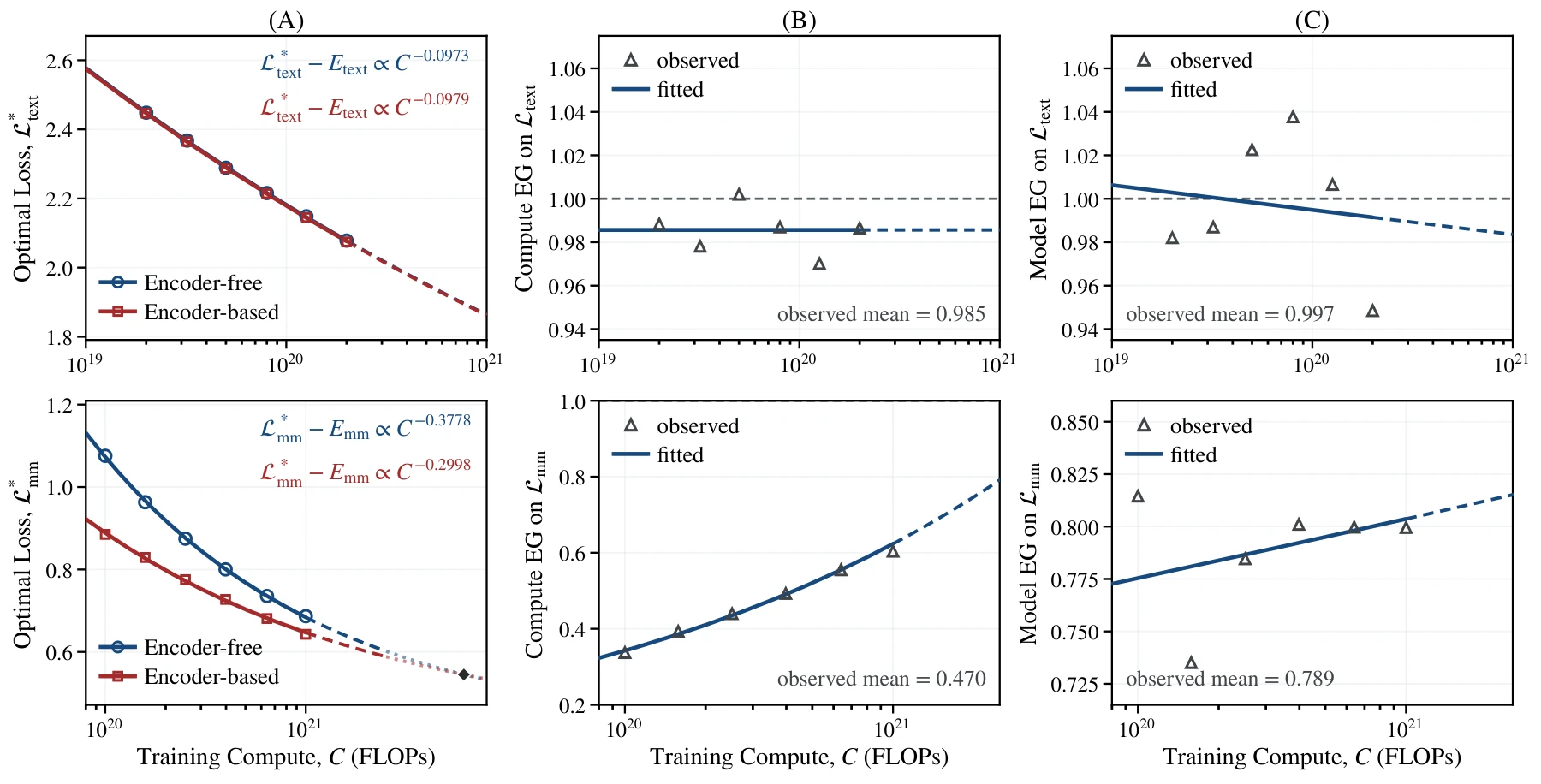
More tokens at a fixed model size
Section titled “More tokens at a fixed model size”Overtraining starts at a compute-optimal model for C_base, keeps M fixed and multiplies its token count by k. Actual compute is kC_base. Substitution into the separable loss gives a multiplier g(k) on the reducible loss. At fixed actual compute, write the multiplier as g(k)k^γ; forgetting this change of axis can reverse an efficiency interpretation.
The idealized derivation gives g(k)=[β+αk⁻ᵝ]/(α+β). The paper instead fits empirical multipliers while keeping E, K and γ fixed. At k=5 these are 0.645 for encoder-free and 0.692 for encoder-based. At the largest fitted budget, the reported multimodal EGᶜ changes from 0.62 to 0.52, and EGᴹ from 0.80 to 0.74. More tokens help loss, but do not erase the relative benefit of allocating more capacity to the encoder-free decoder.
- Paper: §3.2.2 — 2609.35457v1
- Paper: Appendix D; A.3 — 2609.35457v1
Training signals and the decoding protocol
Section titled “Training signals and the decoding protocol”Pretraining uses a 1:1 text/multimodal mixture, sequence length 4096, Muon and 2000 warmup steps. Batch size and learning rate vary by decoder scale, using an internal scaling rule; each paired comparison uses identical hyperparameters. The loss is next-text-token prediction. Visual tokens receive gradients through their influence on predicted text. These details do not provide a complete public reproduction recipe.
Downstream evaluation applies no additional training. All checkpoints share 3-shot examples and prompts. Each example uses at most 192 visual tokens, the query at most 768, and the full prompt at most 4096 tokens. Multiple-choice and yes/no tasks use highest answer likelihood; open answers use greedy decoding for up to 32 tokens, with no external OCR.
- Paper: Appendix A.3–A.4 — 2609.35457v1
- Paper: Appendix G.2 — 2609.35457v1
A loss drop and a visual-attention change
Section titled “A loss drop and a visual-attention change”Figure 7 shows an initially slow encoder-free loss decline followed by a sharper drop. For the analyzed 8B model, layer-12 attention mass on visual tokens rises from 0.217 to 0.645 across the selected checkpoints. The authors hypothesize a feedback loop: weak visual features attract little attention, but useful features receive more learning signal. This is an interpretation of correlated measurements, not an isolated causal intervention.
- Paper: Figure 7; §3.3 — 2609.35457v1
Read Figure 7
Section titled “Read Figure 7”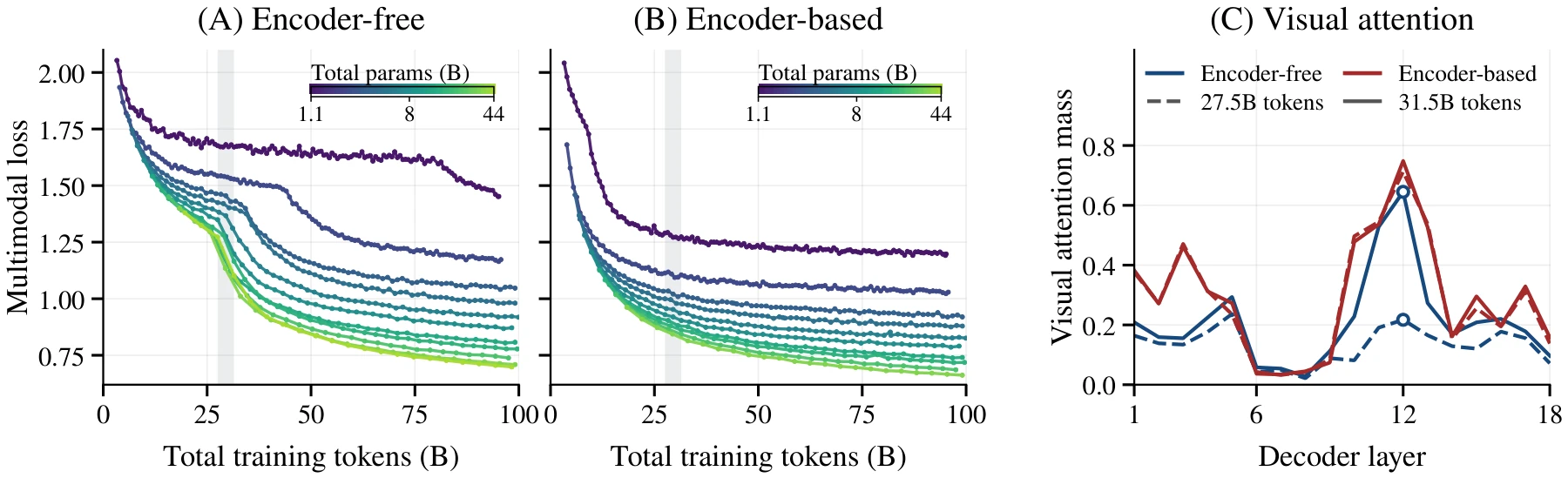
Locate the computation without overclaiming its meaning
Section titled “Locate the computation without overclaiming its meaning”Visual tokens diverge from their input representations earlier in the encoder-free decoder, while text trajectories remain similar. Figure 9 measures cosine similarity to layer 0, not semantic accuracy. Appendix E repeats the pattern at several depths. Expert-load probes in Figure 10 find stronger visual routing concentration when modalities are separated; the aggregate can hide it. A larger MaxVio does not identify what an expert represents.
The causal-mask ablation retains a multimodal model-allocation exponent of 0.557, compared with 0.570 for bidirectional image attention. It supports the allocation shift beyond a mask-only explanation. The reported causal-versus-bidirectional efficiency ratios use causal as the target, so their direction must not be confused with the encoder-free-versus-based ratios above.
- Paper: Figures 9–10 — 2609.35457v1
- Paper: Appendix E.2 — 2609.35457v1
Read Figure 10
Section titled “Read Figure 10”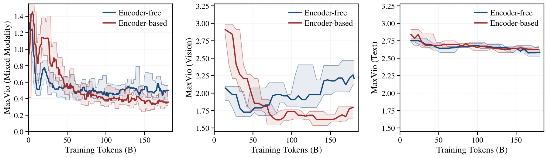
Read Figure 9
Section titled “Read Figure 9”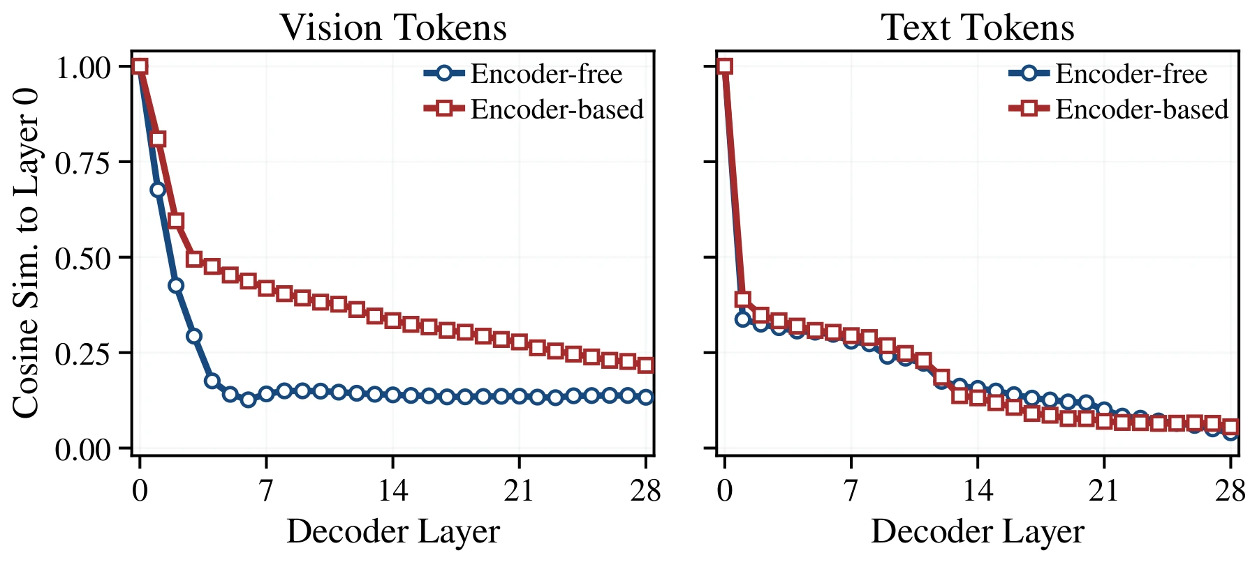
An average gap remains on downstream benchmarks
Section titled “An average gap remains on downstream benchmarks”At about 100B training tokens, Table 6 reports the following unweighted averages over 11 tasks in the same 3-shot protocol. The mean combines different metrics, including accuracy, relaxed accuracy, ANLS and VQA consensus. It is not one unified accuracy score. The gap narrows overall, but not monotonically at every model size or on every task.
Individual counterexamples matter: on CV-Bench at 6.1B-A425M, encoder-free scores 46.9 and encoder-based 42.5. The paper’s statement that encoder-free remains behind should be read as the aggregate trend, not a universal per-benchmark ordering.
| Total / active parameters | Based | Free |
|---|---|---|
| 6.1B / 425M | 43.5 | 35.5 |
| 8B / 577M | 51.9 | 40.5 |
| 13B / 922M | 55.2 | 44.1 |
| 16B / 1B | 53.6 | 43.8 |
| 22B / 1.6B | 57.7 | 48.7 |
| 33B / 2.2B | 57.7 | 51.2 |
- Paper: Table 6; Appendix G — 2609.35457v1
Read Figure 20
Section titled “Read Figure 20”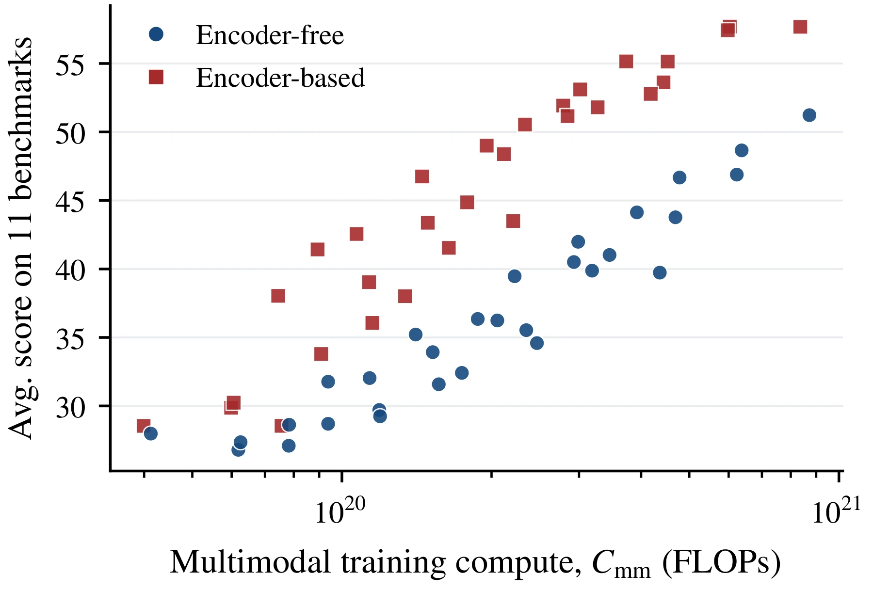
What this does not establish
Section titled “What this does not establish”Which assumptions can move the forecast?
Section titled “Which assumptions can move the forecast?”The two fits share a floor E per objective. The fitted multimodal floor is 0.403, but six frontier points over one decade do not determine the true asymptote. Perturbing this floor by ±10% shifts the k=1 crossover to [4.8, 9.0]×10²¹ FLOPs. This is a sensitivity range, not a confidence interval. The conditional bootstrap uses 4000 paired residual resamples; for k=5 it keeps the already fitted overtraining multipliers fixed.
A held-out multimodal forecast over 2.5× compute has signed loss errors of −0.01% for encoder-free and +2.19% for encoder-based. This useful short-range check does not validate the more distant crossover. The fixed encoder, MoE topology, mixture and preprocessing also limit transfer to other settings. Jointly scaling the encoder is a different allocation problem.
Under full current-training compute accounting, Appendix C reports encoder-based exponents a=0.273 and γ=0.362. The authors do not fit a new numerical crossover under that convention. Do not mix that exponent with the decoder-only crossover and present the result as a measured total-cost threshold.
- Paper: Appendix B.2–B.4 — 2609.35457v1
- Paper: Appendix C — 2609.35457v1
What this changes in a reading of visual tokenizers
Section titled “What this changes in a reading of visual tokenizers”The result separates visual-token count from representation quality. Equal counts do not give equal visual priors. It also suggests that removing an encoder reallocates computation to decoder layers and experts. That is a reason to investigate architecture and allocation together, not a prescription to delete a working visual encoder at a small budget.
Check your understanding
Section titled “Check your understanding”Does a predicted crossover near 10²² FLOPs mean encoder-free models already win?
No. The main multimodal fit stops at 10²¹ FLOPs, and parity is extrapolated under fixed encoder size and a shared loss floor. Downstream average scores still trail in the evaluated range.
Sources and next steps
Section titled “Sources and next steps”Original teaching diagrams and snippets are identified separately from attributed paper figures. Paper reports, implementation observations, and analytical examples are distinguished. No research model runs in this page.