Vision Transformers Need Registers

An interactive field guide

Why do some image positions become global scratch space? Follow the evidence, then trace the added tokens.

Before this article: ViT · Semantic representations

What was already possible

A patch token can stop behaving like a patch

A ViT starts with one vector per image patch. After attention, each vector can contain information from the whole image. A grid-shaped output therefore does not guarantee that every position preserves its original local pixels. CLS is a separate learned readout token. A register is another learned input vector, intended to provide internal workspace.

DINO learns visual representations by matching teacher and student predictions across image views. CLIP-style methods align images with text; DeiT uses class labels. Registers are an architectural addition that the paper studies across these training objectives. They are not a new self-supervised loss or a quantization codebook.

What changes, and why

Read from left to right. Select a module to connect its role, tensor shape, and calculation. Snippets are teaching pseudocode. Sources provide the paper method or audited implementation.

1. Insert learned registers into the shared encoderSee the stage equations below2. Discard workspace outputs, not image positionsSee the stage equations below

Insert learned registers into the shared encoder

Let N be the number of patches, D the feature width and R the number of registers. The input has N+R+1 positions. Register initial values are shared across images, but their activations change with each image through attention. The same Transformer blocks process CLS, registers and patches together.

z = concat(cls, patch_embed(image))
z = z + interpolated_positions
z = concat(z[:, :1], registers, z[:, 1:])
z = transformer(z)

Training state: Static source inspection; training state is discussed below.

$$Z_0=[c; r_1;\ldots;r_R;p_1;\ldots;p_N]\in\mathbb R^{(N+R+1)\times D}$$

Step-by-step explanation: Insert learned registers into the shared encoder

Discard workspace outputs, not image positions

After the final normalization, CLS is at index 0, registers occupy [1,1+R), and image patches occupy [1+R,N+R+1). Only patch features should be reshaped into the spatial grid. Including register vectors in this reshape breaks the correspondence between sequence indices and image positions.

normalized = norm(z)
cls = normalized[:, 0]
reg = normalized[:, 1:1+R]
patch = normalized[:, 1+R:]
image_grid = patch.reshape(B, H_patch, W_patch, D)

Training state: Static source inspection; training state is discussed below.

$$\Delta P=RD,\qquad \rho_{\rm scores}=\frac{(N+R+1)^2}{(N+1)^2}$$

Step-by-step explanation: Discard workspace outputs, not image positions

Inspect the pinned source

$$N_{\rm encoder}=N+R+1,\quad N_{\rm image\ output}=N$$

The evidence behind the workspace hypothesis

The paper finds a small set of high-norm output patch vectors. In the analyzed DINOv2-g case, 2.37% exceed a chosen norm threshold of 150. This threshold is a diagnostic choice for that model. It is not a universal detector. The outliers often correspond to locally redundant background patches.

Linear probes provide two separate observations: outlier tokens recover local position and pixels less well, but predict image-level labels better than ordinary patches. The authors interpret this as reuse of spatial positions for global computation. This is an explanation supported by experiments, not a proof that every large-norm vector is harmful.

$$\|z_i\|_2=\sqrt{\sum_{d=1}^{D}z_{i,d}^2},\qquad a_{ij}=\operatorname{softmax}_j(q_i^Tk_j/\sqrt{d_h})$$

Norm and attention are different quantities. Q/K projections, normalization and vector direction also affect attention. Smooth feature maps and better task scores must be checked separately.

Insert learned registers into the shared encoder

Teaching diagram · Registers: shared computation, separate readout Read each named row from left to right. Rows show distinct pathways or comparison cases. · Method sourceSelect the image to inspect it at full size.

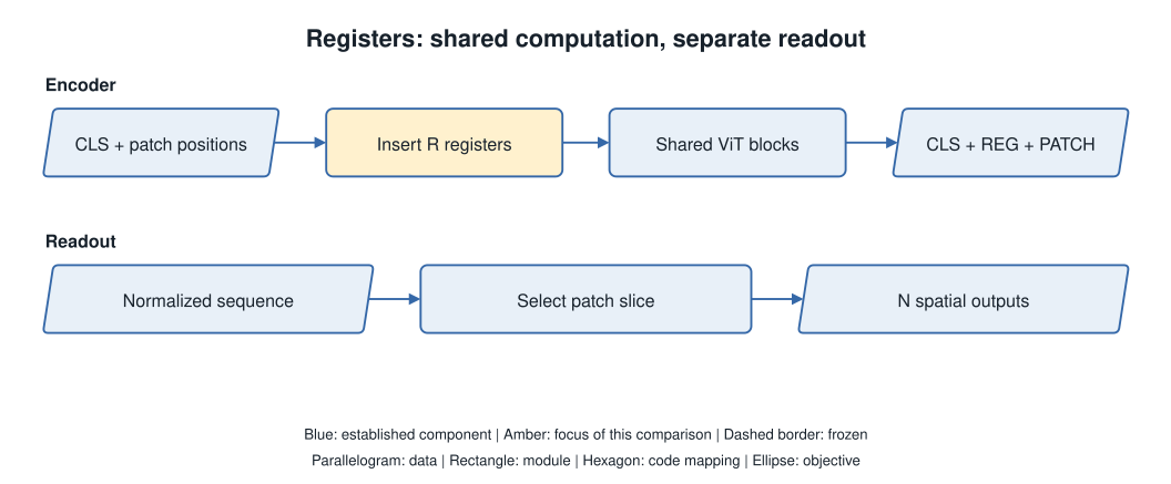
Let N be the number of patches, D the feature width and R the number of registers. The input has N+R+1 positions. Register initial values are shared across images, but their activations change with each image through attention. The same Transformer blocks process CLS, registers and patches together.

In the pinned DINOv2 code, absolute positions are first added to CLS and patches. Registers are then inserted after CLS. The paper figure draws a different token order; the code order is used in this walkthrough. Existing memory-token work already supplied the general mechanism. This paper adds the visual diagnosis and controlled evidence for this remedy.

$$Z_0=[c; r_1;\ldots;r_R;p_1;\ldots;p_N]\in\mathbb R^{(N+R+1)\times D}$$

z = concat(cls, patch_embed(image))
z = z + interpolated_positions
z = concat(z[:, :1], registers, z[:, 1:])
z = transformer(z)

• Pinned DINOv2 implementation — prepare_tokens_with_masks

Work through the mechanism

Discard workspace outputs, not image positions

Teaching diagram · Registers add positions; merging removes positions Read each named row from left to right. Rows show distinct pathways or comparison cases. · Method sourceSelect the image to inspect it at full size.

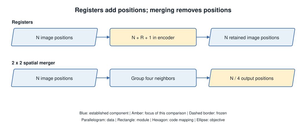
After the final normalization, CLS is at index 0, registers occupy [1,1+R), and image patches occupy [1+R,N+R+1). Only patch features should be reshaped into the spatial grid. Including register vectors in this reshape breaks the correspondence between sequence indices and image positions.

For 256 patches and four registers, the encoder processes 261 positions and returns the same 256-position image grid. Four width-768 input vectors add 3072 parameters. The attention-score matrix grows from 257² to 261² entries per head. This small calculation does not include projections, MLPs or hardware effects.

$$\Delta P=RD,\qquad \rho_{\rm scores}=\frac{(N+R+1)^2}{(N+1)^2}$$

normalized = norm(z)
cls = normalized[:, 0]
reg = normalized[:, 1:1+R]
patch = normalized[:, 1+R:]
image_grid = patch.reshape(B, H_patch, W_patch, D)

Add workspace; keep the image grid

Analytical example: 16×16=256 patches, width 768, and one CLS. Change the register count to inspect sequence structure and attention-score entries. This does not simulate feature quality or training.

Register count

4

CLS × 1REG × 4PATCH × 256

Quantity	Result
Backbone sequence length	261
Retained image positions	256
Python patch slice	[:, 5:261, :]
Added learned parameters	3072
Attention-score entries per head	68121
Entry ratio to R=0	1.0314

Reset

The output slice follows the pinned DINOv2 order: CLS → REG → PATCH. The cost ratio applies only to the attention matrix, not total FLOPs or latency.

Training is not sampling

Train with the changed sequence; inspect the actual controls

The experiments train models with registers. Appending untrained vectors to an existing checkpoint is not the reported procedure. The study uses DeiT-III ViT-B and DINOv2 ViT-L on ImageNet-22k, and OpenCLIP ViT-B/16 on a licensed Shutterstock image–text corpus. These are different training settings.

Most experiments use four registers; the count ablation includes 0, 1, 2, 4, 8 and 16. The appendix also enables antialiasing for DINOv2 position interpolation. A faithful comparison records this setting, the backbone size, training data, readout type and downstream protocol. A register-count slider cannot reproduce these training runs.

Reported evidence, not a local reproduction

Setting	Metric	Value	Interpretation
DINOv2 → +reg, Table 2	ADE20k mIoU	46.6 → 47.9	Frozen-feature linear evaluation
DINOv2 → +reg, Table 3	VOC2007 CorLoc	35.3 → 55.4	LOST
OpenCLIP → +reg, Table 3	VOC2007 CorLoc	38.8 → 37.1	A counterexample to universal improvement

What this does not establish

What this changes for reconstruction research

LOST object discovery improves for DINOv2 but becomes slightly worse for OpenCLIP in the reported comparison. Removing artifacts is therefore not a guarantee of universal gains. The local linear pixel probe is not a full image decoder. The paper does not establish that registers improve RAE reconstruction.

For UAR, first check which tokens the frozen encoder returns and which positions the decoder reads. Then test a matched encoder/decoder comparison if needed. Registers are not TiTok compressed latent slots: this design keeps the original patch grid and adds internal positions.

• RAE: retained patch features
• Original Figure 6 and paper

Check your understanding

Does discarding register outputs mean they did no work?

No. They exchange information through all shared blocks before the output selection.

Sources and next steps

• Vision Transformers Need Registers · 2309.16588v2
• Method / pinned implementation source
• Visual tokenizers in multimodal models

Return to the learning map

Original teaching diagrams and snippets are identified separately from attributed paper figures. Paper reports, implementation observations, and analytical examples are distinguished. No research model runs in this page.